Graph Theory: Part II (Linear Algebra)
This is the second part in my series on graph theory. Part I included the basic definitions of graph theory, gave some concrete examples where one might want to use graph theory to tackle a problem, and concluded with some common objects one finds doing graph theory.
I'm going to cover three things in this post: vector spaces, linear transformations and matrices, and eigenvectors and eigenvalues.
Vector Spaces
Linear algebra is the study of vector spaces and and their transformations. No good mathematical text can begin without definitions, so lets dive in:
Definition. Let R be the real numbers. A vector space over the reals is a set V and two binary operations +: V×V → V and ·: R×V → V, called vector addition and scalar multiplication, respectively, which satisfy the following
(V,+) is an Abelian group.
- Scalar multiplication distributes over vector addition
Formally, α·(v+w) = α·v + α·w for all α ∈ R and v,w ∈ V.
- Vector addition distributes over scalar multiplication
Formally, (α + β)·v = α·v + β·v for all α,β ∈ R and v ∈ V
- Scalar multiplication is compatible with vector addition
Formally, α·(β·v) = (αβ)·v for all α,β ∈ R and v ∈ V
- Scalar multiplication has an identity element
Formally, 1·v = v for all v ∈ V, where 1 is the multiplicative identity.
These properties aren't arbitrary, even though they might look like it. The most common vector space is n-dimensional Euclidean space Rn. R2 is the Cartesian plane we grew up with in grade school and R3 is the three-dimensional space we live in every day.
A vector is an element of a vector space. For x ∈ Rn we write x = (x1, x2, ..., xn), i.e., an ordered tuple of n components. For example, (1,2,3) is an element of R3, as is (√2, 5/3, 2.12).
Let's work in R3. Take v = (1,0,0) and u = (1,1,0). Then v+u = (1+1, 1+0, 0+0) = (2,1,0). That is, addition on R3 is just coordinate-wise addition from R. Scalar multiplication works the same way, so that √3 · (1,10,0) = (√3,10√3,0).
Note. If we're just talking about some abstract vector v in some vector space V over the reals then we refer to the ith coordinate of v as vi.
Linear Transformations and Matrices
Any time you see a mathematical object you should immediately ask yourself, "What are the transformations of this object?" In linear algebra the transformations between vector spaces are called linear transformations (boring, eh?). The definition:
Definition. Let V,W be vector spaces over the reals. A function v: V → W is a linear transformation if it satisfies the following conditions:
- f(v+u) = f(v) + f(u) for all v,u ∈ V
- f(α·v) = α·f(v) for all α ∈ R and v ∈ V
It turns out that every linear transformation can be written as a matrixYeah, yeah, the matrix representation is only unique up to a choice of basis.. Remember those guys from high-school algebra?
Matrices are nice because matrix multiplication corresponds to the composition of linear transformations. That is, let V be a vector space over the reals and let f and g be linear transformations on V whose matrices are A and B respectively. Then, if v ∈ V, we have (A · B)v = f(g(v)). Matrix multiplication is a well-defined, computationally simple operation, where as the composition of linear transformations is comparatively difficult.
I don't want to write a full-on tutorial about multiplying matrices, so I recommend reading the Wikipedia article on the subject. Here's an example of a 3×2 matrix. All of the entries are assumed to be real numbers.

This takes as its input a three-dimensional vector and outputs a two-dimensional vector. In general, an m×n matrix takes as its input an m-dimensional vector and outputs an n-dimensional vector.
Definition. Let A be an m×n matrix over the reals. Then the entry in the ith row and jth column is denoted as aij. One might even write A = (aij).
Definition. Let A be an m×n matrix over the reals. The transpose of A, denoted AT, is the matrix B defined by bij = aji, i.e., the matrix in which the rows and columns are swapped.
The transpose is important for all sorts of things, as we'll see.
Eigenvalues and Eigenvectors
Eigenvalues and eigenvectors are two of the most important objects in linear algebra. They are defined as follows.
Definition. Let A be a square n×n matrix and let v ∈ Rn. v is an eigenvector of A if there exists a real number λ such that
 λ is called an eigenvalue of A and v is the eigenvector corresponding to λ
Who cares about eigenvectors? They're useful for all sorts of things. Calculating a webpage's PageRank, for example, is really a problem of finding a certain eigenvector. You can read about algorithms to calculate eigenvalues, but I'll cover more of that ground in Part III.
For now, just keep this idea in your head. We're going to be doing something very much like PageRank to calculate a person's standing in a social network.
Graphs and Matrices
So far I've not even mentioned graphs, so you're probably wondering what the hell any of this has to do with graph theory. It turns out every graph has several associated matrices that are very useful for analyzing the properties of that graph.
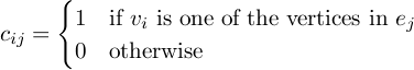
Definition. Let G be a graph with n vertices and m edges, i.e., V = {v1, ..., vn} and E = {e1, ..., em}. The incidence matrix of G is the m×n matrix C(G) = (cij) defined by
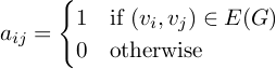
Definition. Let G be a graph with n vertices, V = {v1, ..., vn}. The adjacency graph of G is the n×n square matrix A(G) = (aij) defined by
Definition. Let G be an undirected graph with n vertices. The degree matrix of G, D(G), is the matrix defined by
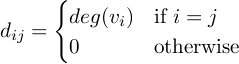
These are the three basic matrices associated with a graph. The incidence matrix encapsulates vertex-edge relationships, the adjacency matrix encapsulates vertex-vertex relationships, and the degree matrix encapsulates information about the degrees. For a concrete example consider the cycle graph C4: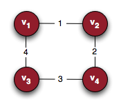
Here are the corresponding matrices: 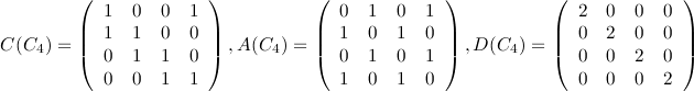
There's one last matrix that is worth knowing.
Definition. Let G be a graph. The Laplacian matrix or graph Laplacian for G is defined as L(G) = D(G) - A(G), where D is the degree matrix and A is the adjacency matrix.
Conclusion
It turns out that lots of information about the graph is stored in these matrices. From these graphs we can calculate things like the number of spanning trees, the algebraic connectivity, etc. Most of these are well-defined eigenvalue problems, and so become computationally feasible.
In Part III we'll use these matrices to tackle the problem of influence or prestige in social networks.