Hypothesis Testing: The Basics
Say I hand you a coin. How would you tell if it's fair? If you flipped it 100 times and it came up heads 51 times, what would you say? What if it came up heads 5 times, instead?
In the first case you'd be inclined to say the coin was fair and in the second case you'd be inclined to say it was biased towards tails. How certain are you? Or, even more specifically, how likely is it actually that the coin is fair in each case?
Hypothesis Testing
Questions like the ones above fall into a domain called hypothesis testing. Hypothesis testing is a way of systematically quantifying how certain you are of the result of a statistical experiment.
In the coin example the "experiment" was flipping the coin 100 times. There are two questions you can ask. One, assuming the coin was fair, how likely is it that you'd observe the results we did? Two, what is the likelihood that the coin is fair given the results you observed?
Of course, an experiment can be much more complex than coin flipping. Any situation where you're taking a random sample of a population and measuring something about it is an experiment, and for our purposes this includes A/B testing.
Let's focus on the coin flip example understand the basics.
The Null Hypothesis
The most common type of hypothesis testing involves a null hypothesis. The null hypothesis, denoted H0, is a statement about the world which can plausibly account for the data you observe. Don't read anything into the fact that it's called the "null" hypothesis — it's just the hypothesis we're trying to test.
For example, "the coin is fair" is an example of a null hypothesis, as is "the coin is biased." The important part is that the null hypothesis be able to be expressed in simple, mathematical terms. We'll see how to express these statements mathematically in just a bit.
The main goal of hypothesis testing is to tell us whether we have enough evidence to reject the null hypothesis. In our case we want to know whether the coin is biased or not, so our null hypothesis should be "the coin is fair." If we get enough evidence that contradicts this hypothesis, say, by flipping it 100 times and having it come up heads only once, then we can safely reject it.
All of this is perfectly quantifiable, of course. What constitutes "enough" and "safely" are all a matter of statistics.
The Statistics, Intuitively
So, we have a coin. Our null hypothesis is that this coin is fair. We flip it 100 times and it comes up heads 51 times. Do we know whether the coin is biased or not?
Our gut might say the coin is fair, or at least probably fair, but we can't say for sure. The expected number of heads is 50 and 51 is quite close. But what if we flipped the coin 100,000 times and it came up heads 51,000 times? We see 51% heads both times, but in the second instance the coin is more likely to be biased.
Lack of evidence to the contrary is not evidence that the null hypothesis is true. Rather, it means that we don't have sufficient evidence to conclude that the null hypothesis is false. The coin might actually have a 51% bias towards heads, after all.
If instead we saw 1 head for 100 flips that would be another story. Intuitively we know that the chance of seeing this if the null hypothesis were true is so small that we would be comfortable rejecting the null hypothesis and declaring the coin to (probably) be biased.
Let's quantify our intuition.
The Coin Flip
Formally the flip of a coin can be represented by a Bernoulli trial. A Bernoulli trial is a random variable X such that
That is, X takes on the value 1 (representing heads) with probability p, and 0 (representing tails) with probability 1 - pOf course, 1 can represent either heads or tails so long as you're consistent and 0 represents the opposite outcome.
Now, let's say we have 100 coin flips. Let Xi represent the ith coin flip. Then the random variable
The Statistics, Mathematically
Say you have a set of observations O and a null hypothesis H0. In the above coin example we were trying to calculate
We can use whatever level of confidence we want before rejecting the null hypothesis, but most people choose 90%, 95%, or 99%. For example if we choose a 95% confidence level we reject the null hypothesis if
The Central Limit Theorem is the main piece of math here. Briefly, the Central Limit Theorem says that the sum of any number of re-averaged identically distributed random variables approximates a normal distribution.
Remember our random variables from before? If we let
But by the central limit theorem we also know that p approximates a normal distribution. This means we can estimate the standard deviation of p as
Wrapping It Up
Our null hypothesis is that the coin is fair. Mathematically we're saying
Here's the normal curve:
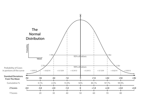
A 95% level of confidence means we reject the null hypothesis if p falls outside 95% of the area of the normal curve. Looking at that chart we see that this corresponds to approximately 1.98 standard deviations.
The so-called "z-score" tells us how many standard deviations away from the mean our sample is, and it's calculated as
The numerator is "p - 0.50" because our null hypothesis is that p = 0.50. This measures how far the sample mean, p, diverges from the expect mean of a fair coin, 0.50.
The Data
Let's say we flipped three coins 100 times each and got the following data.
| Data for 100 Flips of a Coin | |||
|---|---|---|---|
| Coin | Flips | Pct. Heads | Z-score |
| Coin 1 | 100 | 51% | 0.20 |
| Coin 2 | 100 | 60% | 2.04 |
| Coin 3 | 100 | 75% | 5.77 |
Using a 95% confidence level we'd conclude that Coin 2 and Coin 3 are biased using the techniques we've developed so far. Coin 2 is 2.04 standard deviations from the mean and Coin 3 is 5.77 standard deviations.
When your test statistic meets the 95% confidence threshold we call it statistically significant.
This means there's only a 5% chance of observing what you did assuming the null hypothesis was true. Phrased another way, there's only a 5% chance that your observation is due to random variation.
Recap
Hypothesis testing is a way of systematically quantifying how certain you are of the result of a statistical experiment. You start by forming a null hypothesis, e.g., "this coin is fair," and then calculate the likelihood that your observations are due to pure chance rather than a real difference in the population.
The confidence interval is the level at which you reject the null hypothesis. If there is a 95% chance that there's a real difference in your observations, given the null hypothesis, then you are confident in rejecting it. This also means there is a 5% chance you're wrong and the difference is due to random fluctuations.
The null hypothesis can be any mathematical statement and the test you use depends on both the underlying data and your null hypothesis. In our coin flipping example the underlying data approximated a normal distribution and we wanted to test whether the observed proportion of heads was different enough to be significant. In this case we were measuring the sample mean.
We can measure anything, though: the sample variance, correlation, etc. Different tests needs to be used to determine whether these are statistically significant, as we'll see in coming articles.
What's Next?
Now that we understand the innards of hypothesis testing we can apply our knowledge to A/B tests to determine whether new features actually effect user behavior. Until then!